The Chaos Monkey Controversy: Why Overuse is Killing Developer Productivity

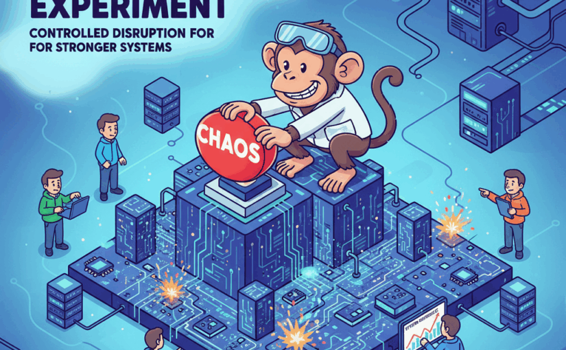
In the world of Site Reliability Engineering (SRE), few tools have sparked as much debate as Netflix’s Chaos Monkey. What started as an innovative approach to building resilient systems has become a lightning rod for controversy, dividing the engineering community into passionate camps. After years of watching teams struggle with its implementation, I’m convinced that the tool’s widespread misuse has created more problems than it solved.

The Promise vs. Reality

Netflix introduced Chaos Monkey in 2014 with a simple premise: randomly terminate instances in production to force teams to build more resilient systems. The idea was sound – if your system can’t handle the unexpected failure of a single component, it’s not truly robust. But somewhere between Netflix’s careful, strategic implementation and the broader industry adoption, something went wrong.

The evidence is everywhere. Reddit discussions in r/sre are filled with horror stories of cascading failures triggered by poorly timed Chaos Monkey deployments. HackerNews threads document teams spending more time recovering from simulated failures than actually improving their systems. As one frustrated developer put it: “Chaos Monkey causes chaos, it does not fix it.”

The Case Against Overuse

The critics’ arguments are compelling and backed by real-world evidence:

Reduced Developer Productivity: Constant, unpredictable deployments disrupt development workflows. Teams report spending excessive time rolling back changes and restoring services instead of building new features. When your developers are in perpetual recovery mode, innovation suffers.

False Sense of Security: Perhaps more dangerously, frequent disruptions create complacency. Teams become so accustomed to recovering from simulated failures that they lose focus on preventative measures. The perception of resilience becomes skewed – surviving artificial chaos doesn’t guarantee handling real-world incidents.

Operational Overhead Explosion: Every Chaos Monkey deployment requires investigation, analysis, and often rollback procedures. This consumes significant resources that could be better spent on proactive improvements and strategic technical debt reduction.

Misinterpretation of Failure Data: Controlled, short-lived interruptions bear little resemblance to sustained, complex outages. The data collected during Chaos Monkey tests cannot reliably inform long-term architectural decisions because the test environment fundamentally differs from genuine failure scenarios.

The Netflix Model: What Actually Works

Netflix’s original implementation wasn’t the blanket deployment strategy many teams have adopted. Their approach was surgical, strategic, and tied to specific maturity milestones. They deployed Chaos Monkey on reduced scales, focused on services that were already stable, and closely monitored the results.

The key difference? Netflix treated Chaos Monkey as a precision instrument, not a blunt force tool. Their engineers understood that the goal wasn’t to cause disruption – it was to observe system behavior under stress and identify specific weaknesses.

The Middle Ground: Disciplined Chaos

This doesn’t mean Chaos Monkey is inherently flawed. When used correctly, it can provide valuable insights. The critical factors for success include:

Service Maturity Requirements: Deploy only on stable, well-understood services. Using Chaos Monkey on immature systems is like stress-testing a house of cards – you’ll learn it falls down, but not much else.

Controlled Frequency: Deployments should be carefully scheduled and spaced, not constant background noise. Teams need time to implement improvements between tests.

Clear Success Metrics: Define specific learning objectives before each deployment. What exactly are you trying to discover or validate?

Comprehensive Monitoring: Ensure you can observe and analyze the complete impact of each test, not just surface-level metrics.

My Take: Strategy Over Chaos

After witnessing both spectacular failures and genuine successes with Chaos Monkey, I believe the tool’s value lies in its strategic application, not its frequency of use. The teams that succeed with chaos engineering treat it like any other engineering discipline – with careful planning, clear objectives, and disciplined execution.

The controversy surrounding Chaos Monkey ultimately reflects a broader issue in our industry: the tendency to adopt powerful tools without fully understanding their appropriate context and limitations. Netflix built Chaos Monkey for their specific needs, scale, and organizational maturity. The problems arise when teams apply it blindly without considering their own unique circumstances.

Looking Forward

The evolution toward tools like Chaos Gorilla and more sophisticated chaos engineering frameworks shows the industry is learning. We’re moving away from random disruption toward targeted, hypothesis-driven resilience testing. This represents a maturation of the chaos engineering discipline – from “break things and see what happens” to “systematically validate our assumptions about system behavior.”

The lesson isn’t to abandon chaos engineering, but to approach it with the same rigor we apply to any other engineering practice. Used strategically, tools like Chaos Monkey can strengthen systems. Used carelessly, they strengthen nothing but frustration levels.

The choice is ours: embrace disciplined chaos or remain victims of chaotic discipline.

Collecting Datadog APM traces using Grafana Alloy and Tempo

The Problem

Hybrid cloud is the future, but monitoring remains stuck in the past. Many organizations embrace hybrid infrastructure, yet struggle with fragmented observability tools. Why? Because monitoring providers still operate in silos.

One of the primary reasons hybrid monitoring isn’t as prevalent is the challenge of instrumentation. Many cloud providers offer their own monitoring solutions. Instrumentation libraries are often incompatible with one another, making cross-platform integration difficult.

The good news? With OpenTelemetry, Grafana, and Datadog, hybrid monitoring is becoming easier and more flexible. 🚀

The Solution

One promising development is the rise of open-source, vendor-neutral instrumentation frameworks like OpenTelemetry.

In essence, open standards are reducing incompatibility issues and allowing “a vendor-agnostic approach to get data from the sources you need to the observability service of your choice.”

A step toward solving the hybrid cloud monitoring challenge came when Grafana introduced the otelcol.receiver.datadog component.

Now, with otelcol.receiver.datadog, Grafana users can ingest and process Datadog telemetry directly within OpenTelemetry pipelines, unlocking several advantages:

  1. Expanding Grafana’s Reach to Datadog Customers
  2. Seamless Integration with OpenTelemetry Pipelines
  3. Avoiding Vendor Lock-in While Retaining Datadog’s Strengths
  4. Cost Optimization by Centralizing Hybrid Monitoring

How it works together?

Requirements

  1. Grafana – for web UI
  2. Grafana Alloy – to receive, process and export telemetry data
  3. Grafana Tempo – to collect and visualize traces from Datadog instrumented apps
  4. Datadog agent – with enabled APM feature
  5. Instrumented application with Datadog trace library

Quick check list:

  1. you have running: Grafana, Alloy and Tempo services
  2. You have running Datadog agents
  3. You have instrumented applications with Datadog trace library
  4. You add Tempo as Datasource in Grafana

Grafana Alloy configuration

The core of the solution is to set up Datadog receiver in Alloy config:

receivers:
datadog:
endpoint: "0.0.0.0:9126"
output:
traces: [otelcol.exporter.otlp.tempo.input]

# I am skipping extra steps which you might want to use to pre-proces data

otelcol:
exporter:
otlp:
tempo:
client:
endpoint: "https://tempo-distributor.example.com:443"
tls:
insecure: false
insecure_skip_verify: true

To avoid ports conflict with Datadog agent we choose 9126 as a port for Alloy Datadog receiver.

Running Alloy as Daemonset with hostNetwork access allow agent to be present on each Node.

alloy:
extraPorts:
- name: "datadog"
port: 9126
targetPort: 9126
protocol: "TCP"

controller:
hostNetwork: true
hostPID: true

service:
internalTrafficPolicy: "Local"

Application set up

Application has to be configured to send APM traces to Node IP:1926.

The Node IP can be extracted form Kubernetes meta information and passed as environment variable:

env:
- name: NODE_IP
valueFrom:
fieldRef:
fieldPath: status.hostIP

Datadog Agent configuration

With Datadog Agent we have two options:

  1. Send traces to Alloy Datadog receiver as addition to Datadog host
  2. Send traces only to Alloy Datadog receiver

With option 1 we assume you are using both Datadog and Grafana solutions in hybrid mode. In that case Datadog agent has to have following configuration:

agents:
containers:
agent:
env:
- name: DD_ADDITIONAL_ENDPOINTS
value: '{"http://alloy-service:9126": ["datadog-receiver"]}'
- name: DD_APM_ADDITIONAL_ENDPOINTS
value: '{"http://alloy-service:9126": ["datadog-receiver"]}'
traceAgent:
enabled: true
env:
- name: DD_ADDITIONAL_ENDPOINTS
value: '{"http://alloy-service:9126": ["datadog-receiver"]}'
- name: DD_APM_ADDITIONAL_ENDPOINTS
value: '{"http://alloy-service:9126": ["datadog-receiver"]}'

For option 2 where traces must go only to Alloy Datadog receiver following configuration might work:

datadog:
apm:
socketEnabled: true # Use the Unix Domain Socket (default). Can be true even if port is enabled.
portEnabled: true # Enable TCP port 8126 for traces.
useLocalService: false

env:
- name: DD_APM_DD_URL
value: "http://alloy-service:9126" # URL for OTel collector’s Datadog trace receiver
- name: DD_APM_NON_LOCAL_TRAFFIC
value: "true"

After all done and agents restarted you can navigate to Explore page in Grafana, select Tempo as datasource and get recent Datadog traces.

Conclusions

  1. Kudos to Grafana and Datadog – Their collaboration on the otelcol.receiver.datadog makes transitioning between monitoring platforms smoother than ever, reducing friction for hybrid observability.
  2. Hybrid Monitoring is the New Normal – Applications no longer rely on a single monitoring provider throughout their lifespan. As infrastructure evolves, businesses will inevitably switch or integrate multiple observability tools.
  3. Stay Agile with Open Standards – Using OpenTelemetry ensures flexibility, allowing teams to adapt their monitoring stack without vendor lock-in, keeping observability seamless across hybrid and multi-cloud environments.

By embracing open standards, organizations can future-proof their monitoring strategies while ensuring complete visibility across their hybrid infrastructure. 🚀

Grafana a new look

As much as l like managed monitoring solutions it’s hard not to be excited about setting up your own platform based on Prometheus Grafana stack and save some bucks for the company.

After 5 years of using proprietary solutions I am again on the way to get into Grafana world.

Here I want to wrap up what I learnt so far about Grafana.

Big ecosystem of tools

The biggest change for me is ecosystem of projects which supports almost all imaginable monitoring needs.

  • For Logs: Loki and Promtail
  • For Traces: Tempo
  • For Profiling: Peryscope
  • For open telemetry collecting: Alloy
  • For eBPF: Beyla
  • For Synthetics: Prometheus BlackBox and K6 API
  • and many more

Automated Deployment process

A lot was done in the deployment process where using Helm charts you can get it up and running in a minutes.

All that comes with scalability and high availability in mind.

Though you would need to connect and customize each component, it’s still can be just a Helm configuration change.

Huge ecosystem of Components to simplify instrumentation

It’s clear your code has to be instrumented to be observable. Grafana and their Open Source community developed a number of tools to make it easy and simple:

  1. Compatible receivers for big providers like Datadog
  2. New discovery methods like eBPF
  3. No code way of instrumentation like sidecar container

And a lot more see the Alloy components section to get started.

New fresh UI

Grafana Logs and Metrics get new look.

You can see multiple logs and metrics on the same page.

Summary

It’s cool, it’s fresh and it’s a lot of fun to use!

Filebeats configuration for Kubernetes

filebeat.autodiscover:
  providers:
  - type: kubernetes
    node: ${NODE_NAME}
    hints.enabled: true
    hints.default_config:
      type: container
      paths:
        - /var/log/containers/*${data.kubernetes.container.id}.log

What’s so cool about above configuration

Filebeat Autodiscover

When you run applications on containers, they become moving targets to the monitoring system. Autodiscover allows you to track them and adapt settings as changes happen.

The Kubernetes autodiscover provider watches for Kubernetes nodes, pods, services to start, update, and stop.
As well it recognise a lot of additional labels and statuses related to Kubernetes objects.

Hints based autodiscover

Filebeat supports autodiscover based on hints from the provider. The hints system looks for hints in Kubernetes Pod annotations or Docker labels that have the prefix co.elastic.logs. As soon as the container starts, Filebeat will check if it contains any hints and launch the proper config for it. Hints tell Filebeat how to get logs for the given container.

Type Container

Use the container input to read containers log files.

This input searches for container logs under the given path, and parse them into common message lines, extracting timestamps too. Everything happens before line filtering, multiline, and JSON decoding, so this input can be used in combination with those settings.

Conclusions

Kubernetes logs autodiscovery and JSON decoding provide very good visibility into log stream. Labels and JSON log fields are properly named and parsed. Using ES and Kibana we can search through logs with easy queries and filter by fields.

References

Integrating Flask with Jaeger tracing on Kuberentes

Distributed applications and microservices required high level of observability. In this article we will integrate a Flask micro framework with Jaeger tracing tool. All code will be deployed to Kubernetes minikube cluster.

Flask

Let’s build a simple task manager service using Flask framework.

Code

tasks.py

from flask import Flask, jsonify
app = Flask(__name__)

@app.route('/')

tasks = {"tasks":[
        {"name":"task 1", "uri":"/task1"},
        {"name":"task 2", "uri":"/task2"}
    ]}

def  root():
	"Service root"
	return  jsonify({"url":"/tasks")
                     
@app.route('/tasks')
def  tasks():
	"Tasks list"
	return  jsonify(tasks)

if __name__ == '__main__':
  "Start up"
  app.run(debug=True, host='0.0.0.0',port=5000)
Continue reading Integrating Flask with Jaeger tracing on Kuberentes

Making simple Splunk Nginx dashboard

As a DevOps guy I often do incident analysis, post deployment monitoring and usual logs checks. If you also is using Splunk as me when let me show for you few effective Splunk commands for Nginx logs monitoring.

Extract fileds

To make commands works Nginx log fields have to be extracted into variables.
Where are 2 ways to extract fields:

  1. By default Splunk recognise “access_combined” log format which is default format for Nginx. If it is your case congratulations nothing to do for you!
  2. For custom format of logs you will need to create regular expression. Splunk has built in user interface to extract fields or you can provide regular expression manually.

field_extractor

Website traffic over time and error rate

Unexpected spike in traffic or in error rate are always first thing to look for. Following command build a time chart with response codes. Codes 200/300 is your normal traffic and 400/500 is errors.

timechart count(status) span=1m by status

Website traffic in Splunk

Response time

How do you know if your website running slowly?
For response time I suggest to use 20, 85 and 95 percentile as metrics.
You also can think of average response time metric, but low average response time doesn’t show that website is OK, so I am not using that metric in the query.

timechart perc20(request_time), perc85(request_time), perc95(request_time) span=1m

Response time in Splunk

Traffic by IP

Checking which IPs are most popular is a good way to spot bad guys or misbehaving bot.

top limit=20 clientip

Traffic by IP with splunk

Top of error page

Looking for pages which produce most errors like 500 Internal Server Error or not found pages like 404? Following two queries give you exactly that information.
Top error pages

search status >= 500 | stats count(status) as cnt by uri, status | sort cnt desc

Top 40x error pages

search status >= 400 AND status < 500 | stats count(status) by uri, status | sort cnt desc

TOP nginx error urls with Splunk

Number of timeouts(>30s) per upstream

When you are using Nginx as a proxy server it is very useful to see if any of upstreams are getting timeouts.
Timeouts could be a symptom for: slow application performance, not enough system resources or just upstream server is down.

search upstream_response_time >= 30 | stats count(upstream_response_time) as upstreams by upstream

Splunk get timeout nginx upstreams

Most time consuming upstreams

Most time consuming upstreams showing which of servers are already overloaded by requests and giving you a hint when application needs to be scaled

stats sum(upstream_response_time), count(upstream) by upstream

Most time consuming upstreams

In conclusion

Splunk functions like timechart, stats and top is your best friends for data aggregation. They are like unix tools – the more tools you know the more easier is to build powerful commands.